The mums2 package is designed to provide researchers with tools to analyze untargeted metabolomics data generated using tandem mass spectroscopy from microbial communities. The overall approach taken to analyze metabolomics data parallels that used to analyze microbial communities using 16S rRNA gene sequencing data. To showcase how to do this, we will demonstrate the package using a previously published dataset that analyzed the metabolome of Botryllus schlosseri.
Process data
Before we begin to analyze the data, we have to process it into a
readable data.frame or object that can be viewed and
transformed. To load your data, we need to run two functions:
import_all_data(), and ms2_ms1_compare().
import_all_data() creates an object reflecting MS1 data,
and ms2_ms1_compare()assigns MS2 spectra to your MS1 data.
At this point, you may need to filter out noise or transform certain
parameters before you can properly analyze your data. To accommodate for
those issues, we have two other functions:
filter_peak_table(), and
change_rt_to_seconds_or_minute().
filter_peak_table() allows your to remove low-quality
features and change_rt_to_seconds_or_minute() allows you to
transform your retention time to minutes or seconds. This allows you to
ensure that the retention time in your MS1 data matches your MS2 data.
Below will explain what each function does in more detail and illustrate
how to go through the pipeline.
Import
The import_all_data() function takes in two files one
describing the peak data (i.e., peak_table) and the other describing the
metadata (i.e., metadata) and converts them into an
mpactr object. The peak_table argument takes a
path to a file describing the peak table data. You can specify the
format of the peak table data using the format argument:
Metaboscape, Progenesis, and None. The value given to the
metadata argument is the path to a CSV-formatted file that
provides information about the samples. In order for your metadata to be
valid, it needs the following columns: “injection”, “sample_code”,
“biological_group”. The values in the “injection” column should match
the sample injection columns inside of the peak_table. “sample_code” is
the ID of your technical replicates. Finally, “biological_group” is the
ID of your biological replicate groups. If you need a deeper
understanding of what format the objects given to the
peak_table and metadata arguments should be
in, take a look at mpactr’s getting started
page.
data <- import_all_data(
  peak_table = mums2_example("boryillus_peaktable.csv"),
  metadata = mums2_example("boryillus_metadata.csv"),
  format = "Progenesis")
Peak Table
Below is the expected format for a Progenesis peak table. It contains samples as columns and features as rows. The feature intensities are expected to be un-normalized.
read_csv(mums2_example("boryillus_peaktable.csv"), skip = 2)
#> Rows: 12822 Columns: 48
#> ── Column specification ────────────────────────────────────────────────────────
#> Delimiter: ","
#> chr (1): Compound
#> dbl (47): m/z, Retention time (min), 221012_DGM_Blank1_1_1_390, 221012_DGM_B...
#>
#> ℹ Use `spec()` to retrieve the full column specification for this data.
#> ℹ Specify the column types or set `show_col_types = FALSE` to quiet this message.
#> # A tibble: 12,822 × 48
#> Compound `m/z` `Retention time (min)` 221012_DGM_Blank1_1_1_39…¹
#> <chr> <dbl> <dbl> <dbl>
#> 1 403.23332 Da 188.08 s 404. 3.13 0
#> 2 387.24448 Da 188.56 s 388. 3.14 8674.
#> 3 387.27587 Da 188.61 s 388. 3.14 0
#> 4 392.23176 Da 190.26 s 393. 3.17 0
#> 5 497.99335 Da 190.74 s 499. 3.18 0
#> 6 279.96160 Da 191.42 s 281. 3.19 0
#> 7 244.13361 Da 203.39 s 245. 3.39 412.
#> 8 447.25451 Da 211.76 s 448. 3.53 0
#> 9 315.05243 Da 214.18 s 316. 3.57 258.
#> 10 436.22069 Da 218.58 s 437. 3.64 6328.
#> # ℹ 12,812 more rows
#> # ℹ abbreviated name: ¹`221012_DGM_Blank1_1_1_390`
#> # ℹ 44 more variables: `221012_DGM_Blank1_1_2_391` <dbl>,
#> # `221012_DGM_Blank1_1_3_392` <dbl>, `221012_DGM_MB1588_3_1_395` <dbl>,
#> # `221012_DGM_MB1588_3_2_396` <dbl>, `221012_DGM_MB1588_3_3_397` <dbl>,
#> # `221012_DGM_MB1589_4_1_398` <dbl>, `221012_DGM_MB1589_4_2_399` <dbl>,
#> # `221012_DGM_MB1589_4_3_400` <dbl>, `221012_DGM_MB1590_5_1_401` <dbl>, …Metadata
The expected format for metadata is below. The metadata file needs to contain at minimum columns for “injection”, “sample_code”, and “biological_group”.
read_csv(mums2_example("boryillus_metadata.csv"))
#> Rows: 45 Columns: 9
#> ── Column specification ────────────────────────────────────────────────────────
#> Delimiter: ","
#> chr (3): Injection, Sample_Code, Biological_Group
#> dbl (1): Injection volume
#> lgl (5): File Text, Sample_Notes, MS method, LC method, Vial_Position
#>
#> ℹ Use `spec()` to retrieve the full column specification for this data.
#> ℹ Specify the column types or set `show_col_types = FALSE` to quiet this message.
#> # A tibble: 45 × 9
#>    Injection      `File Text` Sample_Notes `MS method` `LC method` Vial_Position
#>    <chr>          <lgl>       <lgl>        <lgl>       <lgl>       <lgl>
#>  1 221012_DGM_Bl… NA          NA           NA          NA          NA
#>  2 221012_DGM_Bl… NA          NA           NA          NA          NA
#>  3 221012_DGM_Bl… NA          NA           NA          NA          NA
#>  4 221012_DGM_MB… NA          NA           NA          NA          NA
#>  5 221012_DGM_MB… NA          NA           NA          NA          NA
#>  6 221012_DGM_MB… NA          NA           NA          NA          NA
#>  7 221012_DGM_MB… NA          NA           NA          NA          NA
#>  8 221012_DGM_MB… NA          NA           NA          NA          NA
#>  9 221012_DGM_MB… NA          NA           NA          NA          NA
#> 10 221012_DGM_MB… NA          NA           NA          NA          NA
#> # ℹ 35 more rows
#> # ℹ 3 more variables: `Injection volume` <dbl>, Sample_Code <chr>,
#> #   Biological_Group <chr>
Filter
After importing the data, you can use functions from mpactR to filter
the data. There are four different filters in the mpactR package:
filter_mispicked_ions(), filter_group(),
filter_cv(), and filter_insource_ions() (You
can find more information on mpactR’s website). Although
data filtering is not required, it will help reduce noise and correct
peak selection errors, which will also speed up the analysis.
filtered_data <- data |>
  filter_peak_table(filter_mispicked_ions_params()) |>
  filter_peak_table(filter_cv_params(cv_threshold = 0.2)) |>
  filter_peak_table(filter_group_params(group_threshold = 0.1,
                                            "Blanks")) |>
  filter_peak_table(filter_insource_ions_params())
#> ℹ Checking 12822 peaks for mispicked peaks.
#> ℹ Argument merge_peaks is: TRUE. Merging mispicked peaks with method sum.
#> ✔ 2429 ions failed the mispicked filter, 10393 ions remain.
#> ℹ Parsing 10393 peaks for replicability across technical replicates.
#> ✔ 2229 ions failed the cv_filter filter, 8164 ions remain.
#> ℹ Parsing 8164 peaks based on the sample group: Blanks.
#> ℹ Argument remove_ions is: TRUE.Removing peaks from Blanks.
#> ✔ 2538 ions failed the Blanks filter, 5626 ions remain.
#> ℹ Parsing 5626 peaks for insource ions.
#> ✔ 1082 ions failed the insource filter, 4544 ions remain.

filtered_data
#> Key: <compound, mz, kmd, rt>
#>                     compound        mz     kmd    rt 221012_DGM_Blank1_1_1_390
#>                       <char>     <num>   <num> <num>                     <num>
#>       221012_DGM_Blank1_1_2_391 221012_DGM_Blank1_1_3_392
#>                           <num>                     <num>
#>       221012_DGM_Blank2_1_1_404 221012_DGM_Blank2_1_2_405
#>                           <num>                     <num>
#>       221012_DGM_Blank2_1_3_406
#>                           <num>
#>  [ reached 'max' / getOption("max.print") -- omitted 11 rows and 40 columns ]
Convert retention time to “rt in minutes” or “rt in seconds”
Sometimes an MS2 file will report the retention time in minutes but
the MS1 file will report in seconds. This mismatch will cause incorrect
peak matching between MS1 and MS2 data. The
change_rt_to_seconds_or_minute() function allows users to
synthesize data with different units. Be aware that this function
modifies the mpactr object in place. Therefore, you will
need to call the function again to revert the units. Below will display
a vector of retention time.
get_peak_table(filtered_data)$rt
#> [1] 6.65 8.94 5.89 6.86 6.98
#>  [ reached 'max' / getOption("max.print") -- omitted 4539 entries ]
filtered_data <- change_rt_to_seconds_or_minute(
  mpactr_object = filtered_data, rt_type = "seconds"
)
#> Changing rt values to seconds

filtered_data
#> Key: <compound, mz, kmd, RTINSECONDS>
#>                     compound        mz     kmd RTINSECONDS
#>                       <char>     <num>   <num>       <num>
#>       221012_DGM_Blank1_1_1_390
#>                           <num>
#>  [ reached 'max' / getOption("max.print") -- omitted 11 rows and 45 columns ]
filtered_data <- change_rt_to_seconds_or_minute(
  mpactr_object = filtered_data, rt_type = "minutes"
)
#> Changing rt values to minutes

filtered_data
#> Key: <compound, mz, kmd, RTINMINUTES>
#>                     compound        mz     kmd RTINMINUTES
#>                       <char>     <num>   <num>       <num>
#>       221012_DGM_Blank1_1_1_390
#>                           <num>
#>  [ reached 'max' / getOption("max.print") -- omitted 11 rows and 45 columns ]
Preprocess MS2 data
We can use a .mgf/.mzxml/.mzml-formatted file to match MS2 spectra to
MS1 peaks. The ms2_ms1_compare() function reads a list of
mgf files and matches them to a MS1 feature based on the mass-to-charge
ratio and retention time tolerance. If there are multiple matches, this
function will select the MS2 spectra with the highest intensity. Keep in
mind that MS2 spectra files are very large, they can be anywhere from 1
MB to 100 GB. Therefore, depending on how big the file is, it might take
a few moments for the function to complete.
ms2_ms1_compare() generates a list of data with two data
frames (ms1_data, ms2_matches), a list
(peak_data), and a character vector (“samples”):
-
ms2_matchesis adata.frameobject that contains five columns:mz,rt,ms1_compound_id,spectra_index, andms2_spectrum_id.mzandrtare reported from the MS2 file as mass-to-charge ratio and retention time, respectively.ms1_compound_idis the compound id that was imported from the MS1 peak_table.spectra_indexmatches the MS2 data with its MS2 spectrum. Finally,ms2_spectrum_idis the generated name to represent your MS2 spectra (combination of your mz and rt). This is necessary to properly compare compounds. Since compounds with similar structures are expected to have similar MS2 patterns, we can use algorithmic techniques to compute the similarity between two spectra. This allows us to generate annotations and cluster similar spectra together. -
ms1_datais adata.frameobject containing the data created by running filtering steps from mpactr. -
peak_datais a list object that is generated fromms2_ms1_compare().peak_datais a collection of MS2 peak list. A peak list a collection of fragment ions, they all have a value to represent their intensity and mass-charge ratio. -
samplesis a character vector named listing the groups/samples contained in thepeak_tablefile.
matched_data <- ms2_ms1_compare(
ms2_files = mums2_example("botryllus_v2.gnps.mgf"),
mpactr_object = filtered_data, mz_tolerance = 5, rt_tolerance = 6)
#> Reading: /home/runner/work/_temp/Library/mums2/extdata/botryllus_v2.gnps.mgf ...
#> 674/4544 peaks have an MS2 spectra.
head(get_ms2_matches(matched_data))
#> mz rt ms1_compound_id spectra_index ms2_spectrum_id
#> 1 1023.533 5.89 1000.54504 Da 353.23 s 1 mz1023.53293rt5.89
#> 2 1002.552 5.89 1001.54432 Da 354.35 s 2 mz1002.55208rt5.89
#> 3 1008.593 5.54 1007.58494 Da 332.99 s 3 mz1008.59344rt5.54
#> 4 515.367 6.40 1028.72044 Da 383.88 s 4 mz515.36698rt6.4
#> 5 1046.580 5.91 1045.57237 Da 354.13 s 5 mz1046.57957rt5.91
#> 6 524.361 6.67 1046.70233 Da 400.23 s 6 mz524.36102rt6.67
head(get_ms1_data(matched_data))
#> Key: <compound, mz, kmd, RTINMINUTES>
#> compound mz kmd RTINMINUTES
#> <char> <num> <num> <num>
#> 1: 1000.05311 Da 399.15 s 1001.060 0.06039 6.65
#> 2: 1000.20067 Da 536.14 s 1001.208 0.20795 8.94
#> 3: 1000.54504 Da 353.23 s 1023.534 0.53397 5.89
#> 4: 1000.55418 Da 411.36 s 1001.561 0.56146 6.86
#> 5: 1000.65345 Da 418.99 s 1001.661 0.66073 6.98
#> 6: 1001.54432 Da 354.35 s 1002.552 0.55160 5.91
#> 221012_DGM_Blank1_1_1_390 221012_DGM_Blank1_1_2_391
#> <num> <num>
#> 1: 0 0
#> 2: 0 0
#> 3: 0 0
#> 4: 0 0
#> 5: 0 0
#> 6: 0 0
#> 221012_DGM_Blank1_1_3_392 221012_DGM_Blank2_1_1_404
#> <num> <num>
#> 1: 0 0.000
#> 2: 0 0.000
#> 3: 0 0.000
#> 4: 0 5560.354
#> 5: 0 0.000
#> 6: 0 0.000
#> 221012_DGM_Blank2_1_2_405 221012_DGM_Blank2_1_3_406
#> <num> <num>
#> 1: 0.000 0.00
#> 2: 0.000 0.00
#> 3: 0.000 0.00
#> 4: 5621.311 4907.17
#> 5: 0.000 0.00
#> 6: 0.000 0.00
#> 221012_DGM_Blank3_1_1_419 221012_DGM_Blank3_1_2_420
#> <num> <num>
#> 1: 0 0
#> 2: 0 0
#> 3: 0 0
#> 4: 0 0
#> 5: 0 0
#> 6: 0 0
#> 221012_DGM_Blank3_1_3_421 221012_DGM_Blank4_1_1_434
#> <num> <num>
#> 1: 0 0.000
#> 2: 0 0.000
#> 3: 0 0.000
#> 4: 0 3961.063
#> 5: 0 1538.230
#> 6: 0 0.000
#> 221012_DGM_Blank4_1_2_435 221012_DGM_Blank4_1_3_436
#> <num> <num>
#> 1: 0.000 0.000
#> 2: 0.000 0.000
#> 3: 0.000 0.000
#> 4: 4465.566 3834.320
#> 5: 1201.261 1180.144
#> 6: 0.000 0.000
#> 221012_DGM_MB1588_3_1_395 221012_DGM_MB1588_3_2_396
#> <num> <num>
#> 1: 0.00 0.00
#> 2: 13693.07 16856.57
#> 3: 0.00 0.00
#> 4: 0.00 0.00
#> 5: 0.00 0.00
#> 6: 0.00 0.00
#> 221012_DGM_MB1588_3_3_397 221012_DGM_MB1589_4_1_398
#> <num> <num>
#> 1: 0.00 0
#> 2: 16332.37 0
#> 3: 0.00 0
#> 4: 0.00 0
#> 5: 0.00 0
#> 6: 0.00 0
#> 221012_DGM_MB1589_4_2_399 221012_DGM_MB1589_4_3_400
#> <num> <num>
#> 1: 0 0
#> 2: 0 0
#> 3: 0 0
#> 4: 0 0
#> 5: 0 0
#> 6: 0 0
#> 221012_DGM_MB1590_5_1_401 221012_DGM_MB1590_5_2_402
#> <num> <num>
#> 1: 0 0
#> 2: 0 0
#> 3: 0 0
#> 4: 0 0
#> 5: 0 0
#> 6: 0 0
#> 221012_DGM_MB1590_5_3_403 221012_DGM_MB1591_6_1_407
#> <num> <num>
#> 1: 0 0
#> 2: 0 0
#> 3: 0 0
#> 4: 0 0
#> 5: 0 0
#> 6: 0 0
#> 221012_DGM_MB1591_6_2_408 221012_DGM_MB1591_6_3_409
#> <num> <num>
#> 1: 0 0
#> 2: 0 0
#> 3: 0 0
#> 4: 0 0
#> 5: 0 0
#> 6: 0 0
#> 221012_DGM_MB1592_7_1_410 221012_DGM_MB1592_7_2_411
#> <num> <num>
#> 1: 0 0
#> 2: 0 0
#> 3: 0 0
#> 4: 0 0
#> 5: 0 0
#> 6: 0 0
#> 221012_DGM_MB1592_7_3_412 221012_DGM_MB1593_8_1_413
#> <num> <num>
#> 1: 0 0.000
#> 2: 0 0.000
#> 3: 0 0.000
#> 4: 0 8178.693
#> 5: 0 0.000
#> 6: 0 0.000
#> 221012_DGM_MB1593_8_2_414 221012_DGM_MB1593_8_3_415
#> <num> <num>
#> 1: 0.000 0.000
#> 2: 0.000 0.000
#> 3: 0.000 0.000
#> 4: 7220.826 5520.573
#> 5: 0.000 0.000
#> 6: 0.000 0.000
#> 221012_DGM_MB1594_9_1_416 221012_DGM_MB1594_9_2_417
#> <num> <num>
#> 1: 0 0
#> 2: 0 0
#> 3: 0 0
#> 4: 0 0
#> 5: 0 0
#> 6: 0 0
#> 221012_DGM_MB1594_9_3_418 221012_DGM_MB1595_10_1_422
#> <num> <num>
#> 1: 0 0.000
#> 2: 0 0.000
#> 3: 0 0.000
#> 4: 0 0.000
#> 5: 0 9122.671
#> 6: 0 0.000
#> 221012_DGM_MB1595_10_2_423 221012_DGM_MB1595_10_3_424
#> <num> <num>
#> 1: 0.000 0.00
#> 2: 0.000 0.00
#> 3: 0.000 0.00
#> 4: 0.000 0.00
#> 5: 9405.939 10668.91
#> 6: 0.000 0.00
#> 221012_DGM_MB1597_11_1_425 221012_DGM_MB1597_11_2_426
#> <num> <num>
#> 1: 15105.36 13140.04
#> 2: 0.00 0.00
#> 3: 168557.48 176505.77
#> 4: 19095.97 20017.36
#> 5: 0.00 0.00
#> 6: 53858.91 49121.79
#> 221012_DGM_MB1597_11_3_427 221012_DGM_MB1598_12_1_428
#> <num> <num>
#> 1: 17551.49 0.00
#> 2: 0.00 0.00
#> 3: 160923.45 0.00
#> 4: 23794.62 45269.16
#> 5: 0.00 0.00
#> 6: 52025.21 0.00
#> 221012_DGM_MB1598_12_2_429 221012_DGM_MB1598_12_3_430
#> <num> <num>
#> 1: 0.00 0.00
#> 2: 0.00 0.00
#> 3: 0.00 0.00
#> 4: 55623.04 39774.37
#> 5: 0.00 0.00
#> 6: 0.00 0.00
#> 221012_DGM_MB1599_13_1_431 221012_DGM_MB1599_13_2_432
#> <num> <num>
#> 1: 13573.71 13245.09
#> 2: 0.00 0.00
#> 3: 153978.06 158672.23
#> 4: 53121.98 50611.88
#> 5: 10114.79 10594.81
#> 6: 41070.83 53104.70
#> 221012_DGM_MB1599_13_3_433 cor
#> <num> <lgcl>
#> 1: 13221.95 TRUE
#> 2: 0.00 TRUE
#> 3: 165991.44 TRUE
#> 4: 70537.56 TRUE
#> 5: 10425.28 TRUE
#> 6: 52851.14 TRUE
get_ms2_peaks_data(matched_data)[1]
#> [[1]]
#> [[1]]$mz
#> [1] 1022.596 1023.534 1024.468 1024.540 1024.590 1025.538 1025.577 1025.880
#> [9] 1026.543
#>
#> [[1]]$intensity
#> [1] 88.035540 3698.286100 37.559235 1735.583300 43.992560 803.445070
#> [7] 159.595730 8.381788 224.810270
get_samples(matched_data)
#> [1] "221012_DGM_Blank1_1_1_390" "221012_DGM_Blank1_1_2_391"
#> [3] "221012_DGM_Blank1_1_3_392" "221012_DGM_MB1588_3_1_395"
#> [5] "221012_DGM_MB1588_3_2_396" "221012_DGM_MB1588_3_3_397"
#> [7] "221012_DGM_MB1589_4_1_398" "221012_DGM_MB1589_4_2_399"
#> [9] "221012_DGM_MB1589_4_3_400" "221012_DGM_MB1590_5_1_401"
#> [11] "221012_DGM_MB1590_5_2_402" "221012_DGM_MB1590_5_3_403"
#> [13] "221012_DGM_Blank2_1_1_404" "221012_DGM_Blank2_1_2_405"
#> [15] "221012_DGM_Blank2_1_3_406" "221012_DGM_MB1591_6_1_407"
#> [17] "221012_DGM_MB1591_6_2_408" "221012_DGM_MB1591_6_3_409"
#> [19] "221012_DGM_MB1592_7_1_410" "221012_DGM_MB1592_7_2_411"
#> [21] "221012_DGM_MB1592_7_3_412" "221012_DGM_MB1593_8_1_413"
#> [23] "221012_DGM_MB1593_8_2_414" "221012_DGM_MB1593_8_3_415"
#> [25] "221012_DGM_MB1594_9_1_416" "221012_DGM_MB1594_9_2_417"
#> [27] "221012_DGM_MB1594_9_3_418" "221012_DGM_Blank3_1_1_419"
#> [29] "221012_DGM_Blank3_1_2_420" "221012_DGM_Blank3_1_3_421"
#> [31] "221012_DGM_MB1595_10_1_422" "221012_DGM_MB1595_10_2_423"
#> [33] "221012_DGM_MB1595_10_3_424" "221012_DGM_MB1597_11_1_425"
#> [35] "221012_DGM_MB1597_11_2_426" "221012_DGM_MB1597_11_3_427"
#> [37] "221012_DGM_MB1598_12_1_428" "221012_DGM_MB1598_12_2_429"
#> [39] "221012_DGM_MB1598_12_3_430" "221012_DGM_MB1599_13_1_431"
#> [41] "221012_DGM_MB1599_13_2_432" "221012_DGM_MB1599_13_3_433"
#> [43] "221012_DGM_Blank4_1_1_434" "221012_DGM_Blank4_1_2_435"
#> [45] "221012_DGM_Blank4_1_3_436"Annotating data
Once you have preprocessed your data, we can start to generate
additional information like molecular formulas and annotations.
compute_molecular_formulas() allows us to generate
molecular formulas and annotate_ms2() allows us to annotate
our data based on reference databases. This allows us to confirm known
features and annotate additional metadata to unknown features. Below
will explain in further detail how these functions can be used.
Molecular formula prediction
mums2 can generate de novo molecular formula
predictions using fragmentation trees. The
compute_molecular_formulas() function uses MS2 data to
generate the most explained molecular formula and return it as a result
(for more information: Fragmentation
Trees). The most explained molecular formula simply means the
molecular formula that is explained by the most peaks in the spectra. In
order to create a fragmentation tree, we generate candidate formulas
that comprise of every possible molecular formula the parent mass can
create (using only CHNOPS). We then look at every mass and intensity
pair inside of the spectra and compute every molecular formula. We then
create a one directional graph based on all the molecular formulas
using. A molecular formula will point to another if it is a sub-formula
of another formula (meaning it contains at most as many atoms as the
parent formula). Finally, we can compute a score for each one of the
nodes using methods like Ring Double Bond equivalents, compute molecular
formula score, etc. It is possible that the function is unable to
compute a molecular formula. In these cases, a value of NA
is returned. Warning messages will be printed if no molecular formula is
generated or there is only one possible molecular formula. Due to the
time this function will take to run, we are going to use a small
dataset.
data_small <- import_all_data(
  peak_table = mums2_example("botryllus_pt_small.csv"),
  metadata = mums2_example("boryillus_metadata.csv"),
  format = "None") |>
    filter_peak_table(filter_mispicked_ions_params()) |>
    filter_peak_table(filter_cv_params(cv_threshold = 0.05)) |>
    filter_peak_table(filter_group_params(group_threshold = 0.1,
                                              "Blanks")) |>
    filter_peak_table(filter_insource_ions_params())
#> ℹ Checking 349 peaks for mispicked peaks.
#> ℹ Argument merge_peaks is: TRUE. Merging mispicked peaks with method sum.
#> ✔ 1 ions failed the mispicked filter, 348 ions remain.
#> ℹ Parsing 348 peaks for replicability across technical replicates.
#> ✔ 283 ions failed the cv_filter filter, 65 ions remain.
#> ℹ Parsing 65 peaks based on the sample group: Blanks.
#> ℹ Argument remove_ions is: TRUE.Removing peaks from Blanks.
#> ✔ 14 ions failed the Blanks filter, 51 ions remain.
#> ℹ Parsing 51 peaks for insource ions.
#> ✔ 1 ions failed the insource filter, 50 ions remain.

matched_data_small <- ms2_ms1_compare(
  ms2_files = mums2_example("botryllus_v2.gnps.mgf"),
  mpactr_object = data_small, mz_tolerance = .5, rt_tolerance = 6)
#> Reading: /home/runner/work/_temp/Library/mums2/extdata/botryllus_v2.gnps.mgf ...
#> 1/50 peaks have an MS2 spectra.


matched_data_small <- compute_molecular_formulas(
  mass_data = matched_data_small, parent_ppm = 3, number_of_threads = 2)
#> Calculating potential molecular formulas...
#> Calculating fragmentation trees...
#> 1/1 chemical formulas were predicted

get_molecular_formula_preds(matched_data_small)
#> [1] "C17H57N13O17P2S3"
Annotations
Beyond predicting the molecular formula, we can also use the
annotate_ms2() function to annotate the data in the
matched_ms2_ms1 object using reference databases. A
reference database can be input as msp files using the
read_msp() function. It returns a reference database that
can be used as an input for the annotate_ms2() function. In
the mums2 package, MS2 spectral similarity can be
determined using either spectral entropy (for more information: Spectral Entropy)
or the GNPS algorithm.
While GNPS uses a modified cosine score to compute similarity between
spectra, spectral entropy takes advantage of the total intensities of
the spectra. The chosen method can be used by supplying either,
gnps_param() or spec_entropy_params(). Using
these two methods, we can effectively generate a collection of
annotations based on the reference databases. We have a small massbank
database provided from MSDial
on 05/12/2026 that is preloaded in the package and can be used to
annotate data.
reference_db <- read_msp(msp_file = mums2_example("massbank_example_data.msp"))
#> Reading: /home/runner/work/_temp/Library/mums2/extdata/massbank_example_data.msp ...

annotations <- annotate_ms2(
  mass_data = matched_data, reference = reference_db,
  scoring_params = modified_cosine_params(0.5), ppm = 1000,
  min_score =  0.1, chemical_min_score = 0, number_of_threads = 2)

annotations[1:5,]
#>             query_ms1_id       query_ms2_id    query_mz query_rt ref_idx
#> 1 1028.72044 Da 383.88 s   mz515.36698rt6.4  515.366980 6.400000    3283
#> 2 1028.72044 Da 383.88 s   mz515.36698rt6.4  515.366980 6.400000    3284
#> 3 1028.72044 Da 383.88 s   mz515.36698rt6.4  515.366980 6.400000    3289
#> 4 1028.72044 Da 383.88 s   mz515.36698rt6.4  515.366980 6.400000    3290
#> 5 1050.56754 Da 368.94 s mz1051.57522rt6.15 1051.575220 6.150000    5777
#>   query_formula chemical_similarity    score collisionenergy instrument
#> 1                          0.000000 0.166047              15
#> 2                          0.000000 0.164341              30
#> 3                          0.000000 0.167768              15
#> 4                          0.000000 0.159757              30
#> 5                          0.000000 0.476564             0.0
#>   instrumenttype                comment  ionmode         ccs
#> 1    LC-ESI-ITFT registered in MassBank Positive 229.5588665
#> 2    LC-ESI-ITFT registered in MassBank Positive 229.5588665
#> 3    LC-ESI-ITFT registered in MassBank Positive 229.5588665
#> 4    LC-ESI-ITFT registered in MassBank Positive 229.5588665
#> 5    LC-ESI-ITFT registered in MassBank Positive          -1
#>                                                                                                                                                                                                           smiles
#> 1                                                                                                                                     CCCC1=NC2=C(C=C(C=C2C)C2=NC3=CC=CC=C3N2C)N1CC1=CC=C(C=C1)C1=CC=CC=C1C(O)=O
#> 2                                                                                                                                     CCCC1=NC2=C(C=C(C=C2C)C2=NC3=CC=CC=C3N2C)N1CC1=CC=C(C=C1)C1=CC=CC=C1C(O)=O
#> 3                                                                                                                                     CCCC1=NC2=C(C=C(C=C2C)C2=NC3=CC=CC=C3N2C)N1CC1=CC=C(C=C1)C1=CC=CC=C1C(O)=O
#> 4                                                                                                                                     CCCC1=NC2=C(C=C(C=C2C)C2=NC3=CC=CC=C3N2C)N1CC1=CC=C(C=C1)C1=CC=CC=C1C(O)=O
#> 5 OCC1O[C@@H](OC2=CC=C(\\C=C\\C(=O)OCC3O[C@@H](OC4=C([O+]=C5C=C(O)C=C(O[C@@H]6OC(CO)[C@@H](O)C(O)[C@@H]6O)C5=C4)C4=CC(O)=C(O)C=C4)[C@@H](O[C@@H]4OC[C@@H](O)[C@@H](O)C4O)C(O)[C@@H]3O)C=C2)[C@@H](O)C(O)[C@@H]1O
#>                      inchikey retentiontime precursortype num.peaks
#> 1 RMMXLENWKUUMAY-UHFFFAOYSA-N                      [M+H]+         2
#> 2 RMMXLENWKUUMAY-UHFFFAOYSA-N                      [M+H]+         4
#> 3 RMMXLENWKUUMAY-UHFFFAOYSA-N                      [M+H]+         2
#> 4 RMMXLENWKUUMAY-UHFFFAOYSA-N                      [M+H]+         5
#> 5 OPWPCWHMCUWCGG-XKYKWVHPSA-O                        [M]+         4
#>                                                                                                                           name
#> 1                                                                                            Telmisartan; LC-ESI-ITFT; MS2; CE
#> 2                                                                                            Telmisartan; LC-ESI-ITFT; MS2; CE
#> 3                                                                                            Telmisartan; LC-ESI-ITFT; MS2; CE
#> 4                                                                                            Telmisartan; LC-ESI-ITFT; MS2; CE
#> 5 Cyanidin 3-O-[2''-O-(xylosyl)-6''-O-(p-O-(glucosyl)-p-coumaroyl) glucoside] 5-O-glucoside; LC-ESI-ITFT; MS2; CE 0.0 eV; [M]+
#>                                     ontology precursormz    formula
#> 1                  Biphenyls and derivatives  515.244153 C33H30N4O2
#> 2                  Biphenyls and derivatives  515.244153 C33H30N4O2
#> 3                  Biphenyls and derivatives  515.244153 C33H30N4O2
#> 4                  Biphenyls and derivatives  515.244153 C33H30N4O2
#> 5 Anthocyanidin 3-O-6-p-coumaroyl glycosides 1051.291974  C47H55O27
Operational Metabolomic Units (OMUs)
Operational Metabolomic Units (OMUs) are clusters of metabolites with
similar MS2 spectral patterns and can be used for numerous analyses. To
properly cluster your data together, you need to generate some
similarity or distance between the features of your data. This is where
our dist_ms2() function comes in. After you generate a
data.frame object containing the distances you can use the
cluster_data() function to create your OMUs.
Calculating distances
We have implemented two different distance calculations to generate
distances between compounds. To generate the distances you can use the
GNPS algorithm (modified_cosine_params()) or spectral
entropy algorithm (spec_entropy_params()). Just like above,
being able to compute the similarity between MS2 spectra is what allows
us to cluster data. We can also use the similarity distances to generate
a data.frame for later use.
dist <- dist_ms2(
  data = matched_data, cutoff = 0.3, precursor_threshold = -1,
  score_params = modified_cosine_params(0.5), min_peaks = 0, number_of_threads = 2)

dist
#>   i j       dist
#> 1 1 2 0.05989299
#> 2 1 3 0.06767390
#> 3 1 5 0.06993205
#>  [ reached 'max' / getOption("max.print") -- omitted 59731 rows ]
Clustering into OMUs
We can now cluster these features based on how similar their MS2
spectra are. Using the output of dist_ms2 and the
matched_ms2_ms1 object, we are able to cluster the features
to generate OMUs using the cluster_data() function. This
function implements the iterative OptiClust
algorithm. This function returns a list object with five slots:
label, abundance, cluster,
cluster_metrics, and iteration_metrics:
- label. Represents the cutoff distance used for the cluster
-
abundance. A
data.frameobject that indicates the absolute abundance of the clusters by sample -
cluster. A
data.frameobject that indicates which features clustered together by cluster ID -
cluster_metrics. A
data.frameobject that includes metrics for how the clusters were formed. -
iteration_metrics. A
data.frameobject that shows how the features were clustered at each iteration.
cluster_results <- cluster_data(
  distance_df = dist, ms2_match_data = matched_data, cutoff = 0.3,
  cluster_method = "opticlust")

cluster_results
#> $label
#> [1] 0.3
#>
#> $abundance
#>                      samples  omu abundance
#> 1  221012_DGM_Blank4_1_2_435 omu1      0.00
#> 2  221012_DGM_Blank4_1_1_434 omu1      0.00
#> 3 221012_DGM_MB1599_13_3_433 omu1  48932.22
#>  [ reached 'max' / getOption("max.print") -- omitted 5442 rows ]
#>
#> $cluster
#>                  feature  omu
#> 1 1028.72044 Da 383.88 s omu1
#> 2 1046.70233 Da 400.23 s omu2
#> 3 1067.55304 Da 352.68 s omu3
#> 4 1072.74610 Da 382.97 s omu4
#> 5 1076.25679 Da 479.00 s omu5
#>  [ reached 'max' / getOption("max.print") -- omitted 116 rows ]
#>
#> $cluster_metrics
#>      label cutoff specificity ppv ttp f1score tn mcc fn fp
#>  [ reached 'max' / getOption("max.print") -- omitted 4 columns ]
#>  [ reached 'max' / getOption("max.print") -- omitted 1 rows ]
#>
#> $iteration_metrics
#>      iter time label num_otus cutoff tp tn fp fn sensitivity
#>  [ reached 'max' / getOption("max.print") -- omitted 7 columns ]
#>  [ reached 'max' / getOption("max.print") -- omitted 5 rows ]
#>
#> attr(,"class")
#> [1] "mothur_cluster"
Now that the metabolomic features have been clustered into OMUs, it
is possible to use the abundance of each OMU across samples to perform
ecological analyses using the
create_community_matrix_object() function followed by the
get_community_matrix() function.
community_w_omus <- create_community_matrix_object(cluster_results)
get_community_matrix(community_w_omus)
#>                                omu1      omu2     omu3      omu4     omu5
#> 221012_DGM_Blank4_1_2_435      0.00      0.00     0.00      0.00     0.00
#>                                omu6     omu7     omu8     omu9     omu10
#> 221012_DGM_Blank4_1_2_435       0.0      0.0     0.00    0.000      0.00
#>  [ reached 'max' / getOption("max.print") -- omitted 44 rows and 111 columns ]
You also have the ability to generate a community matrix object without clustering your data into OMUs. If you are familiar with 16S rRNA gene sequencing analysis, this would be similar to ASVs…
community_wo_omus <- create_community_matrix_object(data = matched_data)
get_community_matrix(community_wo_omus)
#>                            1000.54504 Da 353.23 s 1001.54432 Da 354.35 s
#> 221012_DGM_Blank1_1_1_390                     0.0                   0.00
#>                            1007.58494 Da 332.99 s 1028.72044 Da 383.88 s
#> 221012_DGM_Blank1_1_1_390                    0.00                   0.00
#>                            1045.57237 Da 354.13 s 1046.70233 Da 400.23 s
#> 221012_DGM_Blank1_1_1_390                    0.00                   0.00
#>                            1050.56754 Da 368.94 s 1061.59820 Da 352.58 s
#> 221012_DGM_Blank1_1_1_390                    0.00                    0.0
#>                            1066.55379 Da 352.85 s 1067.55304 Da 352.68 s
#> 221012_DGM_Blank1_1_1_390                     0.0                   0.00
#>  [ reached 'max' / getOption("max.print") -- omitted 44 rows and 664 columns ]
Annotation of OMUs
After your data has been clustered, if you wish to see which OMUs the
annotated features are in, you can supply that to the annotation
function using the cluster_data argument. Doing so will add
a column named OMU to the annotations result data.frame
object. This column will display the OMU the feature is represented
in.
annotations <- annotate_ms2(
  mass_data = matched_data, reference = reference_db,
  scoring_params = modified_cosine_params(0.5), ppm = 1000, min_score = 0.7,
  chemical_min_score = 0, cluster_data = cluster_results, number_of_threads = 2)

annotations[1:5,]
#>             query_ms1_id      query_ms2_id   query_mz query_rt ref_idx
#> 1 1088.53252 Da 351.76 s mz545.27303rt7.97 545.273030 7.970000    3762
#> 2 1088.53252 Da 351.76 s mz545.27303rt7.97 545.273030 7.970000    3768
#> 3  365.28353 Da 397.38 s mz366.29238rt6.11 366.292380 6.110000    6302
#> 4  365.28353 Da 397.38 s mz366.29238rt6.11 366.292380 6.110000    6304
#> 5  368.29309 Da 463.53 s  mz369.2987rt7.73 369.298700 7.730000    6034
#>   query_formula chemical_similarity    score collisionenergy instrument
#> 1                          0.000000 0.810909              15
#> 2                          0.000000 0.805937              15
#> 3                          0.000000 0.711204            10.0
#> 4                          0.000000 0.719118            10.0
#> 5                          0.000000 0.822626
#>   instrumenttype                comment  ionmode         ccs
#> 1    LC-ESI-ITFT registered in MassBank Positive          -1
#> 2    LC-ESI-ITFT registered in MassBank Positive          -1
#> 3      LC-ESI-QQ registered in MassBank Positive 195.1324064
#> 4      LC-ESI-QQ registered in MassBank Positive 195.3074064
#> 5     LC-APPI-QQ registered in MassBank Positive          -1
#>                                                                  smiles
#> 1 OP(O)(=O)OCCC(F)(F)C(F)(F)C(F)(F)C(F)(F)C(F)(F)C(F)(F)C(F)(F)C(F)(F)F
#> 2 OP(O)(=O)OCCC(F)(F)C(F)(F)C(F)(F)C(F)(F)C(F)(F)C(F)(F)C(F)(F)C(F)(F)F
#> 3 CC(C)=CCNC1=C2N(C=NC2=NC=N1)[C@@H]1O[C@H](CO)[C@@H](O)[C@H](O)[C@H]1O
#> 4 CC(C)=CCNC1=C2N=CN([C@@H]3O[C@H](CO)[C@@H](O)[C@H](O)[C@H]3O)C2=NC=N1
#> 5                    CC(C)CCCC(C)C1CCC2C3CC=C4C[C@@H](O)CCC4(C)C3CCC12C
#>                      inchikey retentiontime precursortype num.peaks
#> 1 MIABSAQIFYEDJP-UHFFFAOYSA-N                      [M+H]+         2
#> 2 MIABSAQIFYEDJP-UHFFFAOYSA-N                      [M+H]+         2
#> 3 ORUWKZNXHJIZKV-HDNYONAXSA-N                      [M+H]+         3
#> 4 XEHLLUQVSRLWMH-HDNYONAXSA-N                      [M+H]+         3
#> 5 HVYWMOMLDIMFJA-LBHVWCRMSA-N                  [M-H2O+H]+         2
#>                                                    name
#> 1        Perfluorodecyl phosphate; LC-ESI-ITFT; MS2; CE
#> 2        Perfluorodecyl phosphate; LC-ESI-ITFT; MS2; CE
#> 3 N6-Isopentenyladenine-7-glucoside; LC-ESI-QQ; MS2; CE
#> 4 N6-Isopentenyladenine-9-glucoside; LC-ESI-QQ; MS2; CE
#> 5                      Cholesterol; LC-APPI-QQ; MS2; CE
#>                       ontology precursormz     formula   omu
#> 1         Monoalkyl phosphates  544.980501 C10H6F17O4P omu56
#> 2         Monoalkyl phosphates  544.980501 C10H6F17O4P omu56
#> 3               Glycosylamines  366.177195  C16H23N5O5 omu56
#> 4               Glycosylamines  366.177195  C16H23N5O5 omu56
#> 5 Cholesterols and derivatives  369.351578     C27H46O omu56
OMU-based Ecological Analyses
Because of the variation in total ion intensity across samples, it is
necessary to control for uneven sampling of ions. In ecological
analyses, this is typically performed using rarefaction. Those analyses
anticipate that abundances are counts or whole numbers. However,
intensity values are not whole numbers, they have decimal values.
Therefore, because other tools like vegan will not work
with this type of data, it was necessary to adapt the traditional
rarefaction approach to account for decimal values. In the analyses that
follow, it is necessary to set a threshold value below
which intensities are not included. The default value is 100. To
determine the size parameter in the following
alpha_summary() and dist_shared() functions,
it is helpful to look at the distribution of total ion intensities for
each sample
get_community_matrix(community_w_omus) |>
  rowSums() |>
  sort()
#>  221012_DGM_Blank3_1_2_420  221012_DGM_Blank3_1_3_421
#>                   303998.8                   310580.8
#>  221012_DGM_Blank3_1_1_419  221012_DGM_Blank1_1_2_391
#>                   324211.2                   675179.8
#>  221012_DGM_Blank1_1_3_392  221012_DGM_Blank1_1_1_390
#>                   689332.8                   721682.6
#>  221012_DGM_Blank4_1_2_435  221012_DGM_Blank4_1_1_434
#>                   903126.7                   951002.6
#>  221012_DGM_Blank4_1_3_436  221012_DGM_Blank2_1_3_406
#>                   952071.9                  1053454.3
#>  221012_DGM_Blank2_1_2_405  221012_DGM_Blank2_1_1_404
#>                  1063862.6                  1076876.6
#>  221012_DGM_MB1588_3_1_395  221012_DGM_MB1588_3_3_397
#>                  5059034.9                  5197294.3
#>  221012_DGM_MB1588_3_2_396 221012_DGM_MB1598_12_2_429
#>                  5234123.4                 14144913.4
#> 221012_DGM_MB1598_12_3_430 221012_DGM_MB1598_12_1_428
#>                 14271743.5                 14803909.9
#>  221012_DGM_MB1591_6_1_407  221012_DGM_MB1591_6_3_409
#>                 17226885.5                 18308059.8
#>  221012_DGM_MB1591_6_2_408  221012_DGM_MB1590_5_1_401
#>                 18429174.8                 20222447.4
#>  221012_DGM_MB1590_5_2_402  221012_DGM_MB1593_8_1_413
#>                 20378085.6                 22136160.9
#>  221012_DGM_MB1593_8_2_414  221012_DGM_MB1590_5_3_403
#>                 22717256.1                 23404200.9
#>  221012_DGM_MB1593_8_3_415  221012_DGM_MB1589_4_3_400
#>                 23845593.3                 23984121.1
#>  221012_DGM_MB1589_4_1_398  221012_DGM_MB1589_4_2_399
#>                 24154120.6                 24215611.5
#>  221012_DGM_MB1594_9_1_416  221012_DGM_MB1594_9_2_417
#>                 24362501.1                 26800114.1
#>  221012_DGM_MB1594_9_3_418 221012_DGM_MB1599_13_1_431
#>                 27639693.4                 34810189.5
#> 221012_DGM_MB1599_13_2_432 221012_DGM_MB1595_10_2_423
#>                 35101388.1                 35221428.6
#> 221012_DGM_MB1599_13_3_433 221012_DGM_MB1595_10_1_422
#>                 35619721.0                 35801270.3
#> 221012_DGM_MB1595_10_3_424  221012_DGM_MB1592_7_3_412
#>                 38070863.1                 40131211.4
#>  221012_DGM_MB1592_7_1_410  221012_DGM_MB1592_7_2_411
#>                 42153786.9                 45847532.7
#> 221012_DGM_MB1597_11_2_426 221012_DGM_MB1597_11_1_425
#>                 49222461.0                 51314213.2
#> 221012_DGM_MB1597_11_3_427
#>                 52616171.6
We can see the sample with the lowest intensity is a blank with a
total intensity of 303998.8. We might be tempted to use a
size of 303998. However, that would take a very long time
to run. In our experience such a large value does not yield meaningfully
more precision than using a smaller value. In this case, we would
encourage one to use a value of 40000 as is illustrated in the rest of
this tutorial.
Alpha Diversity
Using your community data, you can calculate alpha diversity metrics. Alpha diversity represents richness or diversity in each sample separately. Within mums2 you can quantify diversity using Simpson’s and Shannon’s diversity indices.
alpha_summary(
  community_object = community_w_omus, size = 40000, threshold = 200,
              diversity_index = c("simpson", "shannon", "richness"),
              subsample = TRUE, number_of_threads = 2) |>
  head()
#>                                               samples   simpson   shannon
#> 221012_DGM_Blank4_1_2_435   221012_DGM_Blank4_1_2_435 0.6218898 0.9725834
#> 221012_DGM_Blank4_1_1_434   221012_DGM_Blank4_1_1_434 0.6334562 1.0036431
#> 221012_DGM_MB1599_13_3_433 221012_DGM_MB1599_13_3_433 0.4263663 0.5557598
#>                            richness
#> 221012_DGM_Blank4_1_2_435      8.59
#> 221012_DGM_Blank4_1_1_434      8.77
#> 221012_DGM_MB1599_13_3_433    12.00
#>  [ reached 'max' / getOption("max.print") -- omitted 3 rows ]
Beta Diversity
Beta diversity represents the dissimilarity between different samples. Beta diversity values can be calculated using community structure metrics (i.e., Bray-Curtis, Theta-YC, Moristia-Horn) or community membership metrics (i.e., Jaccard, Hamming, or Sorenson). With the resulting distance values further analyses are possible. Below are examples use Bray-Curtis distances using unclustered metabolites or OMUs.
bray_no_omus <- dist_shared(community_object = community_wo_omus, size = 40000,
                           threshold = 200, diversity_index = "bray", number_of_threads =  2)
bray_no_omus
#>                            221012_DGM_Blank1_1_1_390 221012_DGM_Blank1_1_2_391
#> 221012_DGM_Blank1_1_2_391                 0.03030542
#>                            221012_DGM_Blank1_1_3_392 221012_DGM_MB1588_3_1_395
#> 221012_DGM_Blank1_1_2_391
#>                            221012_DGM_MB1588_3_2_396 221012_DGM_MB1588_3_3_397
#> 221012_DGM_Blank1_1_2_391
#>                            221012_DGM_MB1589_4_1_398 221012_DGM_MB1589_4_2_399
#> 221012_DGM_Blank1_1_2_391
#>                            221012_DGM_MB1589_4_3_400 221012_DGM_MB1590_5_1_401
#> 221012_DGM_Blank1_1_2_391
#>  [ reached 'max' / getOption("max.print") -- omitted 43 rows and 34 columns ]

bray_w_omus <- dist_shared(community_object = community_w_omus, size = 40000,
                          threshold = 200, diversity_index = "bray", number_of_threads =  2)
bray_w_omus
#>                            221012_DGM_Blank4_1_2_435 221012_DGM_Blank4_1_1_434
#> 221012_DGM_Blank4_1_1_434                0.022657902
#>                            221012_DGM_MB1599_13_3_433
#> 221012_DGM_Blank4_1_1_434
#>                            221012_DGM_MB1599_13_1_431
#> 221012_DGM_Blank4_1_1_434
#>                            221012_DGM_MB1598_12_3_430
#> 221012_DGM_Blank4_1_1_434
#>                            221012_DGM_MB1598_12_1_428
#> 221012_DGM_Blank4_1_1_434
#>                            221012_DGM_MB1597_11_2_426
#> 221012_DGM_Blank4_1_1_434
#>                            221012_DGM_MB1595_10_3_424
#> 221012_DGM_Blank4_1_1_434
#>                            221012_DGM_MB1595_10_2_423
#> 221012_DGM_Blank4_1_1_434
#>                            221012_DGM_MB1597_11_3_427
#> 221012_DGM_Blank4_1_1_434
#>  [ reached 'max' / getOption("max.print") -- omitted 43 rows and 34 columns ]
The output of dist_shared() is a dist
object, which lends itself well to visualization techniques like PCoA
and NMDS and hierarchical clustering.
Visualizations
There are no functions built-in to mums2 for data visualization. Instead, we encourage users to leverage the functionality of ggplot2 and the rest of the tidyverse.
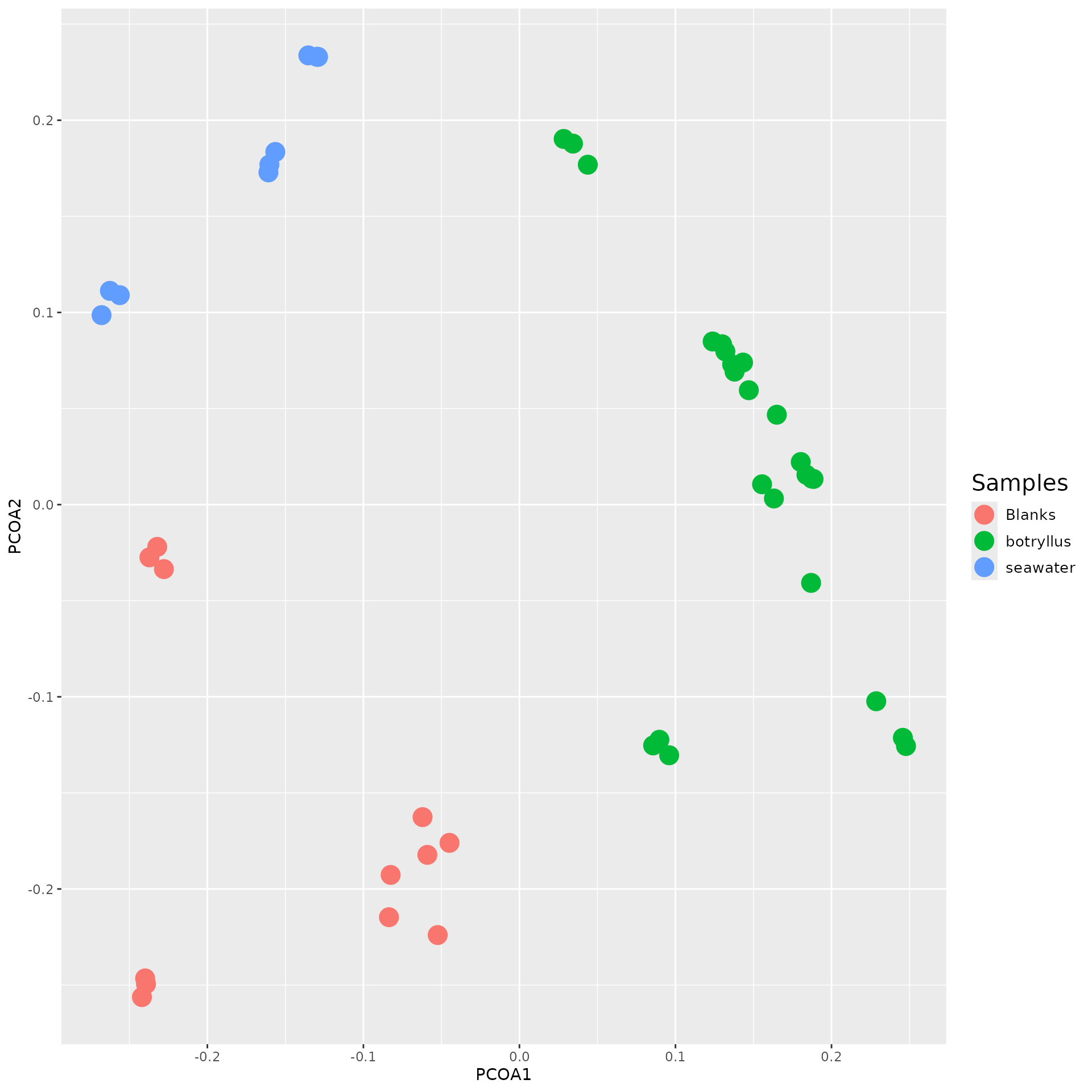
Principal Coordinate Analysis (PCoA)
PCoA is a statistical technique used to show similarities between data. PCOA allows us, in particular, to use the distances generated from our ecological analysis.
pcoa <- cmdscale(bray_w_omus, k = 2, eig = T, add = T)

variance <- round(pcoa$eig*100/sum(pcoa$eig), 1)
colnames(pcoa$points) <- c("pcoa_1", "pcoa_2")

as_tibble(pcoa$points, rownames = "sample") |>
  inner_join(get_metadata(filtered_data), by = c("sample" = "injection")) |>
  ggplot(aes(x=pcoa_1, y = pcoa_2, color = biological_group)) +
    geom_point(size = 5.5) +
    labs(
      x = paste0("PCoA 1 (", variance[1], "%)"),
      y = paste0("PCoA 2 (", variance[2], "%)"),
      color = "Sample type") +
    theme(
      legend.text = element_text(size = 10),
      legend.title = element_text(size = 15)
    )
Hierarchical Clustering
Another visualization approach is to perform hierarchical clustering
using the stats::hclust() function. Hierarchical clustering
generates a tree of samples based on their beta diversity values to show
the similarities of the samples. The results are similar to that of PCoA
but it uses a tree like structure to showcase relationships. It tends to
be easier to look at relationships or clusters using this type of
graph.
old_par <- par(no.readonly = TRUE)
hclust_result <- hclust(bray_w_omus, "average")
par(cex=0.6, mar=c(5, 8, 4, 1))
plot(hclust_result)
par(old_par)Network Plot
Sometimes, it is useful to see a visual map of your annotations. We
can accomplish this using a network plot. By creating a network of data,
we can see which annotations matched certain features. Using
networkD3::simpleNetwork(), we can generate a simple
network plot.
distance_df_annotations <- annotations[, c("query_ms2_id", "name", "score")]

simpleNetwork(
  distance_df_annotations, height="100px", width="100px", zoom = TRUE)
Using Group Averages
Another feature included inside of mums2 is the
ability to run your analysis using group averages. Some researchers
conduct mass spectrometry experiments by running samples in
technical/injection triplicate to account for instrument variability.
Since we know all three injections are from the same vial, we can
average all of these into one group. We can generate group averages by
using the metadata file that was supplied when you imported your data
based on “sample_code”. We can accomplish this by using the
convert_to_group_averages() function.
Below, you can see a copy of the alpha and beta diversity functions we ran above. But this time, we are using group averages.
  matched_avg <- convert_to_group_averages(
  matched_data = matched_data, mpactr_object = filtered_data)

dist_avg <- dist_ms2(
  data = matched_avg, cutoff = 0.3, precursor_thresh = 2,
  score_params = modified_cosine_params(0.5), min_peaks = 0, number_of_threads = 2)

cluster_results_avg <- cluster_data(
  distance_df = dist, ms2_match_data = matched_avg, cutoff = 0.3,
  cluster_method = "opticlust")

annotations_avg <- annotate_ms2(
  mass_data = matched_avg,
  reference = reference_db, scoring_params = modified_cosine_params(0.5),
  ppm = 1000, min_score = 0.6, chemical_min_score = 0,
  cluster_data = cluster_results_avg, number_of_threads = 2)

community_object_avg <- create_community_matrix_object(
  data = cluster_results_avg)
head(get_community_matrix(community_object = community_object_avg), 3)
#>            omu1    omu2 omu3    omu4 omu5 omu6 omu7 omu8 omu9 omu10 omu11 omu12
#> blank3     0.00     0.0    0     0.0    0    0    0    0    0     0     0     0
#> MB1589 23337.03 24115.4    0 14022.7    0    0    0    0    0     0     0     0
#> MB1588     0.00     0.0    0     0.0    0    0    0    0    0     0     0     0
#>        omu13 omu14 omu15    omu16   omu17    omu18 omu19 omu20    omu21
#> blank3     0     0     0     0.00     0.0      0.0     0     0    0.000
#> MB1589     0     0     0 42087.33 10749.4 127599.7     0     0 8942.717
#> MB1588     0     0     0     0.00     0.0      0.0     0     0    0.000
#>           omu22 omu23 omu24    omu25    omu26 omu27    omu28    omu29 omu30
#> blank3    0.000     0     0    0.000     0.00     0     0.00     0.00     0
#> MB1589 7274.027     0     0 5316.441 73722.57     0 67484.12 35960.23     0
#> MB1588    0.000     0     0    0.000     0.00     0     0.00     0.00     0
#>           omu31    omu32    omu33 omu34    omu35 omu36 omu37    omu38 omu39
#> blank3     0.00    0.000     0.00     0     0.00     0     0    0.000     0
#> MB1589 61818.83 8703.846 29907.96     0 28524.01     0     0 8212.385     0
#> MB1588     0.00    0.000     0.00     0     0.00     0     0    0.000     0
#>        omu40 omu41 omu42 omu43 omu44 omu45    omu46 omu47 omu48    omu49 omu50
#> blank3     0     0     0     0     0     0    0.000     0     0     0.00     0
#> MB1589     0     0     0     0     0     0 9891.063     0     0 31016.72     0
#> MB1588     0     0     0     0     0     0    0.000     0     0     0.00     0
#>          omu51 omu52 omu53     omu54 omu55      omu56    omu57     omu58 omu59
#> blank3     0.0     0     0      0.00     0   536344.8     0.00      0.00     0
#> MB1589 18200.5     0     0  60820.68     0 11950209.3 10110.24  98530.36     0
#> MB1588     0.0     0     0 212704.06     0  2761290.9     0.00 479136.87     0
#>        omu60 omu61     omu62    omu63    omu64   omu65 omu66 omu67 omu68 omu69
#> blank3     0     0  71059.94     0.00     0.00     0.0     0     0     0     0
#> MB1589     0     0 578187.41 11067.09 20210.32 11347.3     0     0     0     0
#> MB1588     0     0      0.00     0.00     0.00     0.0     0     0     0     0
#>             omu70 omu71    omu72      omu73      omu74    omu75 omu76    omu77
#> blank3      0.000     0    0.000   65837.39   4293.939     0.00     0     0.00
#> MB1589 210327.208     0 7873.674 5096777.02 217270.654 49602.83     0 67868.33
#> MB1588   6803.707     0    0.000 1098725.26  15809.002 27996.26     0     0.00
#>           omu78 omu79 omu80 omu81     omu82     omu83    omu84     omu85
#> blank3     0.00     0     0     0  101080.8  4267.063     0.00      0.00
#> MB1589 83334.29     0     0     0 2751336.9 28711.179 96614.68  61664.97
#> MB1588     0.00     0     0     0       0.0     0.000     0.00 138083.00
#>            omu86 omu87     omu88    omu89 omu90    omu91    omu92 omu93 omu94
#> blank3  98687.36     0  4669.115     0.00     0     0.00     0.00     0     0
#> MB1589 322682.14     0 23251.863 19642.83     0 57334.46 38534.01     0     0
#> MB1588 260084.95     0     0.000     0.00     0     0.00     0.00     0     0
#>           omu95      omu96    omu97   omu98     omu99 omu100 omu101 omu102
#> blank3     0.00   7709.688      0.0     0.0  37381.96      0      0      0
#> MB1589 62575.24 278049.688 804098.7 37879.9 166117.64      0      0      0
#> MB1588     0.00      0.000      0.0     0.0  26708.77      0      0      0
#>        omu103 omu104 omu105   omu106 omu107    omu108 omu109   omu110 omu111
#> blank3      0      0      0     0.00      0   4068.33      0     0.00      0
#> MB1589      0      0      0 12633.89      0 118577.04      0 38765.94      0
#> MB1588      0      0      0     0.00      0      0.00      0 46022.30      0
#>        omu112 omu113   omu114   omu115 omu116 omu117 omu118 omu119 omu120
#> blank3      0      0     0.00     0.00      0      0      0      0      0
#> MB1589      0      0 73379.17 15677.16      0      0      0      0      0
#> MB1588      0      0 90119.16     0.00      0      0      0      0      0
#>        omu121
#> blank3      0
#> MB1589      0
#> MB1588      0
You can also see how the samples in the matched object have been adjusted based on the information supplied in the metadata file.
# Normal
head(get_samples(matched_data))
#> [1] "221012_DGM_Blank1_1_1_390" "221012_DGM_Blank1_1_2_391"
#> [3] "221012_DGM_Blank1_1_3_392" "221012_DGM_MB1588_3_1_395"
#> [5] "221012_DGM_MB1588_3_2_396" "221012_DGM_MB1588_3_3_397"

# Group Average
head(get_samples(matched_avg))
#> [1] "blank"  "MB1588" "MB1589" "MB1590" "blank1" "MB1591"

# The items in the injection have been converted into the corresponding sample code.
get_metadata(filtered_data)[, c("injection", "sample_code")]
#>                      injection sample_code
#>                         <char>      <char>
#>  1:  221012_DGM_Blank1_1_1_390       blank
#>  2:  221012_DGM_Blank1_1_2_391       blank
#>  3:  221012_DGM_Blank1_1_3_392       blank
#>  4:  221012_DGM_MB1588_3_1_395      MB1588
#>  5:  221012_DGM_MB1588_3_2_396      MB1588
#>  6:  221012_DGM_MB1588_3_3_397      MB1588
#>  7:  221012_DGM_MB1589_4_1_398      MB1589
#>  8:  221012_DGM_MB1589_4_2_399      MB1589
#>  9:  221012_DGM_MB1589_4_3_400      MB1589
#> 10:  221012_DGM_MB1590_5_1_401      MB1590
#> 11:  221012_DGM_MB1590_5_2_402      MB1590
#> 12:  221012_DGM_MB1590_5_3_403      MB1590
#> 13:  221012_DGM_Blank2_1_1_404      blank1
#> 14:  221012_DGM_Blank2_1_2_405      blank1
#> 15:  221012_DGM_Blank2_1_3_406      blank1
#> 16:  221012_DGM_MB1591_6_1_407      MB1591
#> 17:  221012_DGM_MB1591_6_2_408      MB1591
#> 18:  221012_DGM_MB1591_6_3_409      MB1591
#> 19:  221012_DGM_MB1592_7_1_410      MB1592
#> 20:  221012_DGM_MB1592_7_2_411      MB1592
#> 21:  221012_DGM_MB1592_7_3_412      MB1592
#> 22:  221012_DGM_MB1593_8_1_413      MB1593
#> 23:  221012_DGM_MB1593_8_2_414      MB1593
#> 24:  221012_DGM_MB1593_8_3_415      MB1593
#> 25:  221012_DGM_MB1594_9_1_416      MB1594
#> 26:  221012_DGM_MB1594_9_2_417      MB1594
#> 27:  221012_DGM_MB1594_9_3_418      MB1594
#> 28:  221012_DGM_Blank3_1_1_419      blank2
#> 29:  221012_DGM_Blank3_1_2_420      blank2
#> 30:  221012_DGM_Blank3_1_3_421      blank2
#> 31: 221012_DGM_MB1595_10_1_422      MB1595
#> 32: 221012_DGM_MB1595_10_2_423      MB1595
#> 33: 221012_DGM_MB1595_10_3_424      MB1595
#> 34: 221012_DGM_MB1597_11_1_425      MB1597
#> 35: 221012_DGM_MB1597_11_2_426      MB1597
#> 36: 221012_DGM_MB1597_11_3_427      MB1597
#> 37: 221012_DGM_MB1598_12_1_428      MB1598
#> 38: 221012_DGM_MB1598_12_2_429      MB1598
#> 39: 221012_DGM_MB1598_12_3_430      MB1598
#> 40: 221012_DGM_MB1599_13_1_431      MB1599
#> 41: 221012_DGM_MB1599_13_2_432      MB1599
#> 42: 221012_DGM_MB1599_13_3_433      MB1599
#> 43:  221012_DGM_Blank4_1_1_434      blank3
#> 44:  221012_DGM_Blank4_1_2_435      blank3
#> 45:  221012_DGM_Blank4_1_3_436      blank3
#>                      injection sample_code
#>                         <char>      <char>
Combined data frames
mums2 also allows you to view your all of your
generated data together using the
generate_a_combined_table() function. This function will
take your matched object (generated from
ms2_ms1_compare()), your annotations object (generated from
annotate_ms2()) and your cluster data (generated from
cluster_data()) to generate a combined data.frame with all
of the generated data.
# For normal data
generate_a_combined_table(
matched_data = matched_data, annotations = annotations,
cluster_data = cluster_results) |>
head(n = 3)
#> ms1_id ms2_id mz RTINMINUTES omus
#> 1 1000.05311 Da 399.15 s 1001.06039 6.65
#> 2 1000.20067 Da 536.14 s 1001.20795 8.94
#> 3 1000.54504 Da 353.23 s mz1023.53293rt5.89 1023.53397 5.89 omu56
#> annotations 221012_DGM_Blank1_1_1_390 221012_DGM_Blank1_1_2_391
#> 1 <NA> 0 0
#> 2 <NA> 0 0
#> 3 <NA> 0 0
#> 221012_DGM_Blank1_1_3_392 221012_DGM_Blank2_1_1_404 221012_DGM_Blank2_1_2_405
#> 1 0 0 0
#> 2 0 0 0
#> 3 0 0 0
#> 221012_DGM_Blank2_1_3_406 221012_DGM_Blank3_1_1_419 221012_DGM_Blank3_1_2_420
#> 1 0 0 0
#> 2 0 0 0
#> 3 0 0 0
#> 221012_DGM_Blank3_1_3_421 221012_DGM_Blank4_1_1_434 221012_DGM_Blank4_1_2_435
#> 1 0 0 0
#> 2 0 0 0
#> 3 0 0 0
#> 221012_DGM_Blank4_1_3_436 221012_DGM_MB1588_3_1_395 221012_DGM_MB1588_3_2_396
#> 1 0 0 0
#> 2 0 13693.07422 16856.57227
#> 3 0 0 0
#> 221012_DGM_MB1588_3_3_397 221012_DGM_MB1589_4_1_398 221012_DGM_MB1589_4_2_399
#> 1 0 0 0
#> 2 16332.37109 0 0
#> 3 0 0 0
#> 221012_DGM_MB1589_4_3_400 221012_DGM_MB1590_5_1_401 221012_DGM_MB1590_5_2_402
#> 1 0 0 0
#> 2 0 0 0
#> 3 0 0 0
#> 221012_DGM_MB1590_5_3_403 221012_DGM_MB1591_6_1_407 221012_DGM_MB1591_6_2_408
#> 1 0 0 0
#> 2 0 0 0
#> 3 0 0 0
#> 221012_DGM_MB1591_6_3_409 221012_DGM_MB1592_7_1_410 221012_DGM_MB1592_7_2_411
#> 1 0 0 0
#> 2 0 0 0
#> 3 0 0 0
#> 221012_DGM_MB1592_7_3_412 221012_DGM_MB1593_8_1_413 221012_DGM_MB1593_8_2_414
#> 1 0 0 0
#> 2 0 0 0
#> 3 0 0 0
#> 221012_DGM_MB1593_8_3_415 221012_DGM_MB1594_9_1_416 221012_DGM_MB1594_9_2_417
#> 1 0 0 0
#> 2 0 0 0
#> 3 0 0 0
#> 221012_DGM_MB1594_9_3_418 221012_DGM_MB1595_10_1_422
#> 1 0 0
#> 2 0 0
#> 3 0 0
#> 221012_DGM_MB1595_10_2_423 221012_DGM_MB1595_10_3_424
#> 1 0 0
#> 2 0 0
#> 3 0 0
#> 221012_DGM_MB1597_11_1_425 221012_DGM_MB1597_11_2_426
#> 1 15105.3584 13140.04102
#> 2 0 0
#> 3 168557.4844 176505.7656
#> 221012_DGM_MB1597_11_3_427 221012_DGM_MB1598_12_1_428
#> 1 17551.48633 0
#> 2 0 0
#> 3 160923.4531 0
#> 221012_DGM_MB1598_12_2_429 221012_DGM_MB1598_12_3_430
#> 1 0 0
#> 2 0 0
#> 3 0 0
#> 221012_DGM_MB1599_13_1_431 221012_DGM_MB1599_13_2_432
#> 1 13573.70703 13245.09473
#> 2 0 0
#> 3 153978.0625 158672.2344
#> 221012_DGM_MB1599_13_3_433
#> 1 13221.94824
#> 2 0
#> 3 165991.4375
# For group averaged data
generate_a_combined_table(
matched_data = matched_avg, annotations = annotations_avg,
cluster_data = cluster_results_avg) |>
head(n = 3)
#> ms1_id ms2_id mz RTINMINUTES omus
#> 1 1000.05311 Da 399.15 s 1001.06039 6.65
#> 2 1000.20067 Da 536.14 s 1001.20795 8.94
#> 3 1000.54504 Da 353.23 s mz1023.53293rt5.89 1023.53397 5.89 omu56
#> annotations blank MB1588 MB1589 MB1590 blank1 MB1591 MB1592 MB1593
#> 1 <NA> 0 0 0 0 0 0 0 0
#> 2 <NA> 0 15627.3391933333 0 0 0 0 0 0
#> 3 <NA> 0 0 0 0 0 0 0 0
#> MB1594 blank2 MB1595 MB1597 MB1598 MB1599 blank3
#> 1 0 0 0 15265.6285833333 0 13346.9166666667 0
#> 2 0 0 0 0 0 0 0
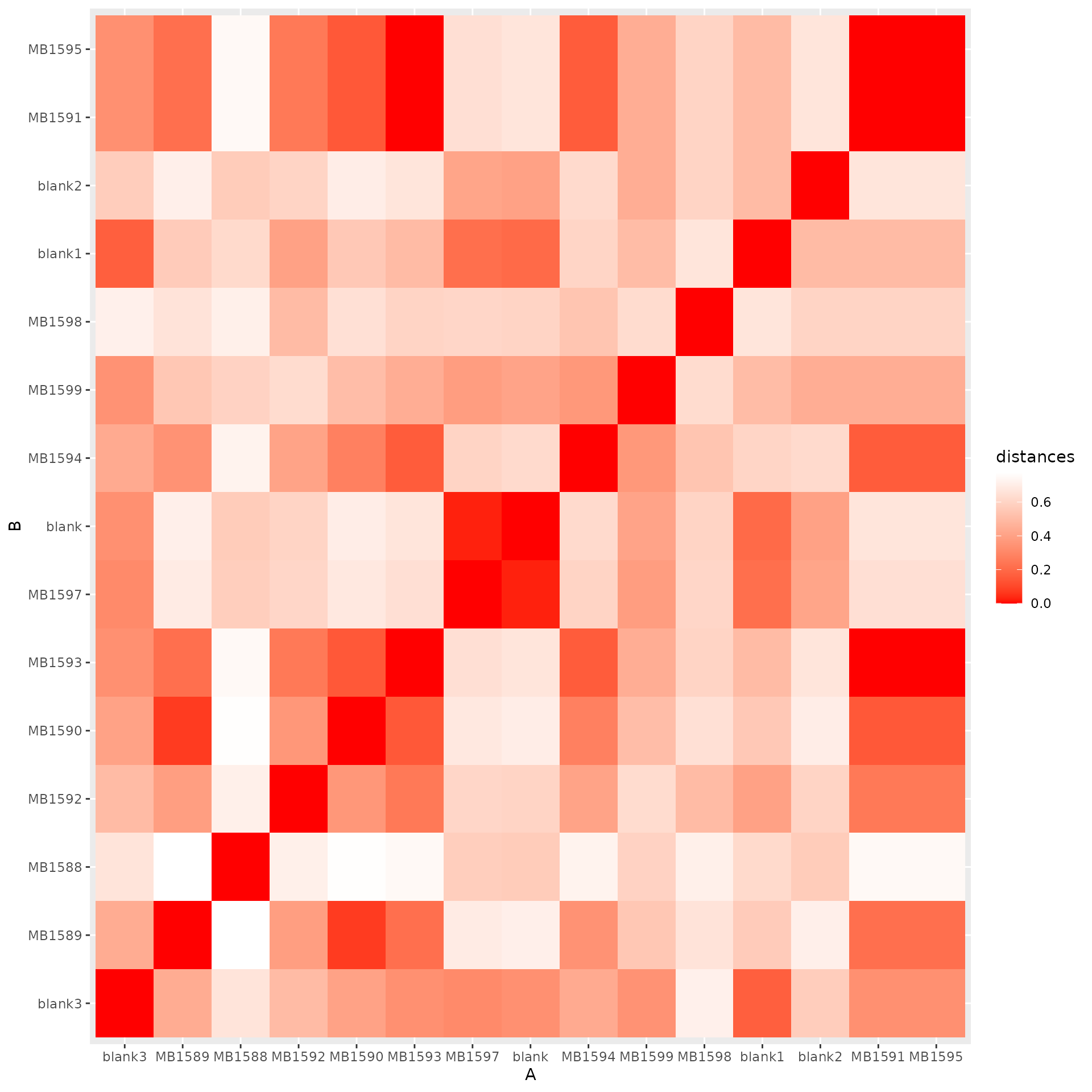
#> 3 0 0 0 168662.234366667 0 159547.2448 0Heat map
Another way to visualize diversity data is to use a heat map. We can easily see how correlated data is between samples with a heatmap.
dist_shared(community_object_avg, 40000, 200, "bray", number_of_threads = 2) |>
  as.matrix() |>
  as_tibble(rownames = "A") |>
  pivot_longer(-A, names_to = "B", values_to = "distance") |>
  ggplot(aes(x = A, y = B, fill = distance)) +
  geom_tile() +
  scale_fill_gradient(low = "#FFFFFF", high="#FF0000") +
  theme(
    axis.text.x = element_text(angle = 90, vjust = 0.5, hjust = 1),
    panel.background = element_blank()
  )
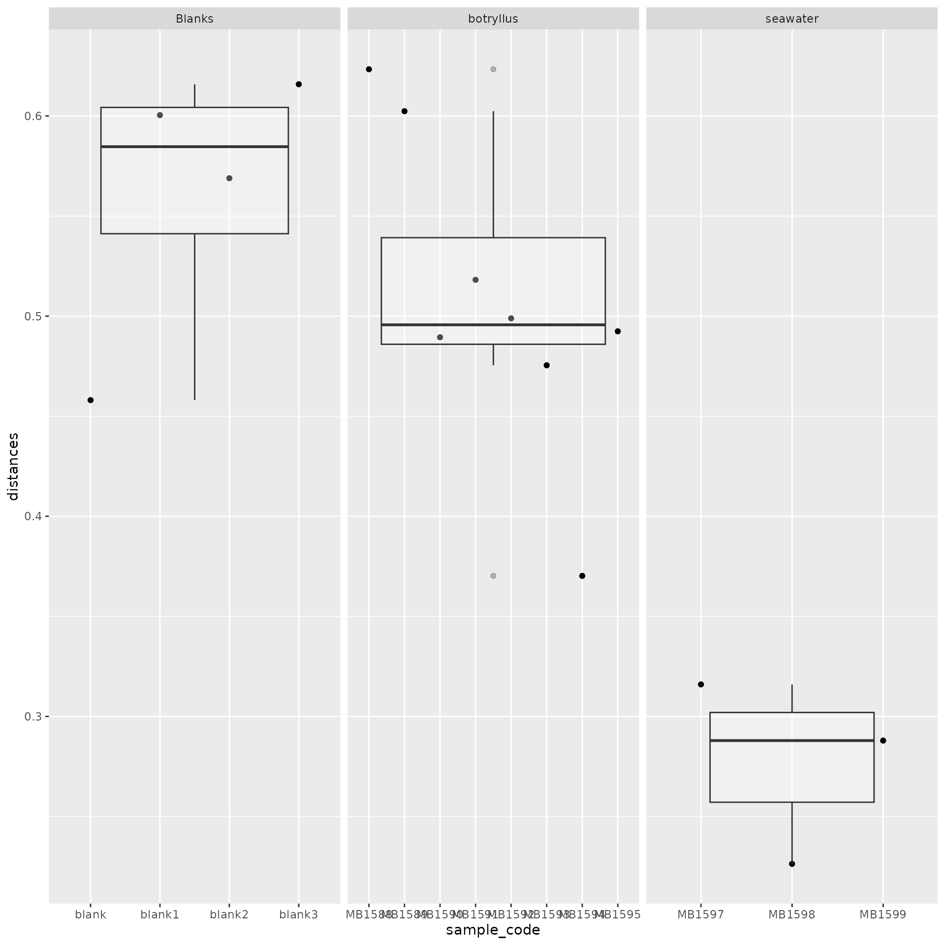
Box Plot
A box and whisker plot can also be used to depict the variation of the data. We can take advantage of this to look at the distributions inside of our generate beta and alpha diversity data. Below is a box plot using alpha diversity.
metadata <- get_metadata(filtered_data)

alpha <- alpha_summary(community_object_avg, 40000, 200, "simpson", number_of_threads = 2)

inner_join(alpha, metadata, by = c("samples" = "sample_code")) |>
  ggplot(aes(x = biological_group, y = simpson)) +
  geom_boxplot(outliers = FALSE, fill = NA, color = "gray") +
  geom_jitter(width = 0.3)  +
  scale_y_continuous(limits = c(0, NA)) +
  theme_classic()